Alternative asset classes are in something of a sweet spot. Not only do they offer the prospect of a diversifying source of return in an environment when bond yields are at historically low levels, but they also provide a new revenue source for active managers. In the current landscape, strategies where passive replication is problematic or impossible provide a particular allure for margin-pressured asset management firms.  Whilst the attention being lavished upon this area is unsurprising there are certain aspects of discussions about such investments, which are troubling and often misleading.

Alternative assets represent a broad church and can encompass anything that falls outside of the core traditional mix of equities and bonds, from private equity to fine wine.  The nebulous nature of this definition means that it is difficult and unfair to discuss the credibility of the grouping in general terms; however, one common feature tends to be the approach to pricing and valuation.  Whereas the majority of traditional assets are regularly traded and marked to market; alternative assets are typically far less liquid and, in the absence of a regularly traded market price, are valued on some form of model / appraisal basis.  This approach to valuation is not a problem in and of itself – there is often no simple answer to appropriately valuing such assets – however, it does have profound implications for how you might express the risks of such strategies and compare them to traditional asset classes.

The first, seemingly obvious, point is that volatility is a woefully inadequate measure of risk for most alternative assets, particularly if used in comparison with public equity returns, for example.  The pricing of any mark to model asset is smoothed; it is largely immune to the vagaries of human behaviour that drive the vacillations of listed assets – imagine the volatility of the S&P 500 if it was valued on a monthly basis based on projected future cash flows.  Volatility has come to be the primary term for how we express investment risk, even where it is inappropriate for the assets in scope.  This incongruence has been exploited by some to suggest that alternative assets in general terms are inherently lower risk, turning a structural limitation* into a sales message.

Deeply intertwined with the issues surrounding volatility and mark to model pricing in alternative assets is the issue of correlation and diversification.  Whilst some alternative assets will have genuinely distinctive attributes when compared to traditional equity / bond portfolios, these should be driven by the underlying economics / cash flow profile of the assets rather than the valuation methodology or liquidity structure.  The most egregious example often comes in the form of some private equity strategies, where a portfolio of private, medium sized companies can be said to offer material diversification benefits compared to a portfolio of public, medium sized companies.  Clearly, the holdings of the two portfolios are highly economically correlated, even if their differential approaches to valuation provide an optical sheen of differentiation.

The narrative supporting alternative assets is often built around the impact that their addition can have on a traditional portfolio (such as a 60/40); whilst there may be merit to this viewpoint, the primary evidence given is often fatuous. The argument tends to run as follows: ‘look at the beneficial Sharpe ratio and volatility impact of adding XYZ alternative strategy to your portfolio’.  Alternative assets exhibit artificially low volatilities and therefore abnormally high Sharpe ratios, they can also appear to have a low correlation to traditional assets – of course they look wonderful when added to a leaden portfolio of equities and bonds.

The problem is that as an industry we have come to use volatility and Sharpe ratio as default metrics for the analysis of traditional portfolios and are now prone to view everything through these frames even when their usage is entirely inappropriate.  Furthermore, given that many asset allocators are assessed on such metrics the rational course of action for them is to game these measures by utilising alternative assets with depressed volatility and low correlations to ‘enhance’ the overall results of their portfolios.

That is not to say that there is no role for alternative assets but any investment case for them should be driven by an understanding of their economic merit and cash flow profile, we should always ask – do arguments around diversification and low volatility make intuitive sense?  Such assets can appear low risk when viewed through a volatility lens – attractive in risk models and optimisations – but such smooth returns can often cloak an unpleasant tail.  Beware the dangers of mistaking pricing and liquidity characteristics for fundamental ones.

—

* As I have previously argued, one indirect benefit of illiquid assets is behavioural – if it is difficult / impossible to trade, we are more likely to stay invested for the long-term.

Imagine you are in a team meeting discussing a potential investment with three colleagues, you ask them how probable it is that your investment thesis for a particular position comes to fruition, each of them states that they see it as ‘likely’.  In an alternate universe, you are in the same situation the only difference being the responses from your colleagues – on this occasion they each say ‘60%’.  Does your colleagues’ shift from a verbal to numeric expression of probability impact your confidence in the investment decision?  A new paper from Robert Mislavsky and Celia Gaertig contends that it would – their research suggests that when we are given numeric probability forecasts we average them and when given verbal forecasts we count them.  A succession of ‘sixty percents’ leads you to a 60% average, whereas a similar number of ‘likely’ responses sees your own view become ‘very likely’.

We often talk in probabilistic terms without realising it – when we state something is ‘likely’ or ‘very likely’ we are expressing some form of view on the probability of an occurrence, although it is admittedly a vague one.  Research around this area has typically focused on the comparison and translation of verbal probability expressions into numeric ones, and vice-versa – when we say something is unlikely, what probability do we actually mean?   As Mislavsky and Gaertig note in their paper, verbal probabilities have the benefit of being clear in their direction (you can tell if it is positive or negative) but suffer from imprecision, whereas numeric probabilities are specific but the direction is not always clear (whether a 45% probability is positive depends on the context).

Mislavsky and Gaertig’s research develops the thinking around this subject by moving on from identifying specific differences between individual verbal and numeric probability expressions, and showing that there is a material change in outcome when we combine a number of verbal probabilities, compared to when we combine a selection of numeric probabilities.  Their research incorporates a range of experiments (7 in total) wherein participants were required to make a decision or predict an outcome after receiving one or two expert forecasts – these forecasts were either both numeric or both verbal.

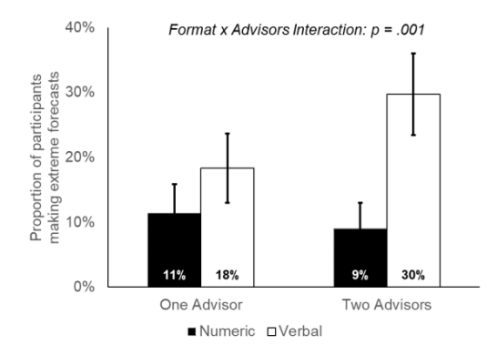
For example, in their second study, participants were provided with some details about a company and asked to judge how likely it was that its share price would be higher in a year’s time.  Some participants received expert guidance from advisers in numeric form and some from advisers in verbal form.  The results of this study – which were consistent with all the experiments carried out in the research –  was that “participants became more likely to make extreme forecasts as they saw additional advisor forecasts in the verbal condition but less likely to do so in the numeric condition”.  We can see this in the chart below:

The predictions of the participants clearly became more extreme when they received an additional verbal forecast but not when an additional numeric forecast was provided.  By ‘extreme forecast’ the authors mean when a participant’s forecast is in excess of that given by either adviser.  Similar results were observed when the study moved from looking at a hypothetical stock price, to predictions of Major League Baseball games with probabilities given by genuine experts.

There is clear evidence from the study that the verbal probabilities lead to a counting process, whereas numeric probabilities are averaged. There are good reasons for both approaches – counting works on the basis that each adviser is providing new information, whereas averaging is prudent if we assume each forecast is founded on the same information.  There is no requirement, however, to associate the different expressions of probability with different processes for their combination – two 60% forecasts could just as easily be driven by different information as two ‘likelys’.  So what is happening?

The authors conclude the paper by reviewing and largely discounting a range of potential explanations (I would urge everyone to read the paper directly).  My best guess of the cause of the phenomenon would be a combination of some of the factors mentioned by the authors, in particular how individuals are liable to perceive numeric and verbal probabilities in different fashions.  Numeric forecasts feel precise and objective, and more consistent with an ‘outside view’ driven by the base rate or reference class – more likely to contain all relevant information.  Contrastingly, verbal probabilities seem personal and subjective, more akin to an ‘inside view’ where an individual providing a forecast will be doing so based on their own unique knowledge or perspective – therefore an additive approach can seem justified.

This idea is pure speculation about which the authors are sceptical, however, whilst the drivers of this contrasting approach to combining probabilities are uncertain; the results, from this initial study at least, are clear, and there is an important lesson for investors to heed.  It is crucial to consider not only the type of guidance and advice we are receive when informing a decision, but how it is being expressed.  This is relevant whether it relates to an individual’s decision using a range of external information sources, or a team based decision making process where we are seeking to synthesise the insights of a number of individuals into a single view.

—

Mislavsky, R., & Gaertig, C. (2019). Combining Probability Forecasts: 60% and 60% Is 60%, but Likely and Likely Is Very Likely. Available at SSRN 3454796.

I have an investment decision to make.  I need to allocate money to a particular asset class and have to decide whether to use a passive market tracker fund to gain exposure or invest with an active manager.  The odds are not in favour of the active option – over the last decade only 10% of managers in the asset class have outperformed the benchmark – however, I have identified a manager with unsurpassable pedigree in the area, a fantastic performance track record and a robust investment process.  Which option should I choose?

The stark contrast of perspectives underpinning this question is an example of what Kahneman and Tversky would label as the ‘outside view’ versus the ‘inside view’[i].  The outside view in this scenario is that 10% of active managers achieve success in the asset class, and is what we can consider to be our base case or reference class – it provides a statistical framework for informing a decision.  My experience of being impressed by a particular manager is the inside view, which is developed using information specific to my individual case which, as Michael Mauboussin notes, may include “anecdotal evidence and fallacious perceptions”[ii].   We can broadly characterise the outside and inside view informing any decision as having the following features:

Our general tendency is to focus on the inside view – we adore narratives, tend to believe that our own experiences are exceptional and are overconfident in our abilities.  Use of the inside view is particularly prevalent in the active asset management industry as, of course, it must be – if something does not work on average then it must be forged on the notion of edge, competitive advantage and exceptionalism.

The inside view is also so much more compelling – those wonderful and usually superfluous stories of active managers gaining an advantage by visiting the factory of a target company (it always seems to be a factory) or meeting management are both diverting and persuasive.  The problem is that they do not change the odds; rather they simply encourage us to forget them.  We often think that the additional insights from detailed research are improving our decisions, but in many cases they are simply making us neglect the base rate (whilst erroneously increasing our confidence)[iii].

Returning to the question with which I began this post; if I select the active manager option then I need to support that decision with one of two claims.  I can argue that the base rate is incorrect and therefore the odds are more favourable than they appear – there is something about historical experience which means it is not representative of the future.  Alternatively, I can accept the probabilities but possess such belief in my active manager selection capabilities that I am not concerned by them.  In most cases we don’t actually make either of these arguments explicitly, we simply ignore the outside view and make the case using our inside view – which is usually sufficiently captivating to overwhelm more prosaic considerations.

This is not to suggest that the inside view is of no merit, but rather it should be used only as a complement or adjustment to the outside view. Our starting point should always be a consideration of the reference class or general evidence that frames a particular scenario.  We can then revise this (usually modestly) if we obtain relevant information that is specific to our case.  A failure to follow this approach means that we will consistently make decisions which ‘feel’ right but where the odds are stacked against us.

—

[i] https://www.mckinsey.com/business-functions/strategy-and-corporate-finance/our-insights/daniel-kahneman-beware-the-inside-view

[ii] Mauboussin, M. J. (2012). Think twice: Harnessing the power of counterintuition. Harvard Business Review Press.

[iii] https://behaviouralinvestment.com/2019/01/09/can-more-information-lead-to-worse-investment-decisions/